

Because I’ve been spending all my time studying lately, the only thing I’ve had time to write is study notes. So I thought that I’d make the most of them, share a bit of my new knowledge with you, and give you a quick crammer’s guide to some of the topics from each of my subjects this semester. The information probably won’t mean a whole lot to you if you’ve never learnt anything about the topic before, but if you have, hopefully, this’ll clear up a few things for you.
This one’s about Network Technologies. This subjects covers the OSI model, IP scheming, data encoding and transmission, flow control, routing and packet switching.
Cyclic Redundancy Check (CRC)
This is a error detection method, which uses a shared pattern and binary division to detect errors in transmissions of data at a binary level. There are two phases to CRC: the sending phase and the receiving phase. Before anything happens, both the sender and receiver must share a pattern, which is a short binary number, which is used during the CRC.
SENDER
1. A string of 0s as long as (the pattern length – 1) is appended to the end of the data string.
2. The new data string is binary divided by the pattern.
Binary division is a pretty strange thing at first, but once you’ve done it a few times, you get use to it. It’s basically just like long division, but binary. You line up the pattern with the data, and cancel out what you can.
1 vs 1 = 0 | 0 vs 0 = 0 | 1 vs 0 = 1
When you run out of digits, you pull down some more, and do it again. And you just repeat that, until you get to the end.
3. Repeat until out of data to divide. You should end up with a remainder the same length as that bunch of 0s we added to the data in the first step.
4. Append the remainder to the original data string, in place of those added 0s.
5. Send off the data!
| _ | _ | _ | _ | _ | _ | _ | _ | _ | _ | _ | _ | _ | _ | ||||||
| 1 | 1 | 0 | 0 | 1 | 1 | ) | 1 | 1 | 1 | 0 | 0 | 0 | 1 | 1 | 0 | 0 | 0 | 0 | 0 |
| ) | 1 | 1 | 0 | 0 | 1 | 1 | ↓ | ↓ | | | | | | | | | | | ||||||
| _ | _ | _ | _ | _ | _ | _ | _ | _ | _ | _ | _ | _ | |||||||
| 0 | 0 | 1 | 0 | 1 | 1 | 1 | 1 | | | | | | | | | | | |||||||
| 1 | 1 | 0 | 0 | 1 | 1 | ↓ | | | | | | | | | |||||||||
| _ | _ | _ | _ | _ | _ | _ | _ | _ | _ | _ | |||||||||
| 0 | 1 | 1 | 1 | 0 | 0 | 0 | | | | | | | | | |||||||||
| 1 | 1 | 0 | 0 | 1 | 1 | ↓ | ↓ | | | | | ||||||||||
| _ | _ | _ | _ | _ | _ | _ | _ | _ | _ | ||||||||||
| 0 | 0 | 1 | 0 | 1 | 1 | 0 | 0 | | | | | ||||||||||
| 1 | 1 | 0 | 0 | 1 | 1 | ↓ | | | ||||||||||||
| _ | _ | _ | _ | _ | _ | _ | _ | ||||||||||||
| 0 | 1 | 1 | 1 | 1 | 1 | 0 | | | ||||||||||||
| 1 | 1 | 0 | 0 | 1 | 1 | ↓ | |||||||||||||
| _ | _ | _ | _ | _ | _ | _ | |||||||||||||
| 0 | 0 | 1 | 1 | 0 | 1 | 0 | |||||||||||||
| _ | _ | _ | _ | _ |
| Remainder = | 11010 |
RECEIVER
1. Received data is binary divided by pattern.
2. Repeat until out of data to divide. You should end up with no remainder. If there’s a remainder. There’s an error.
| _ | _ | _ | _ | _ | _ | _ | _ | _ | _ | _ | _ | _ | _ | ||||||
| 1 | 1 | 0 | 0 | 1 | 1 | ) | 1 | 1 | 1 | 0 | 0 | 0 | 1 | 1 | 1 | 1 | 0 | 1 | 0 |
| ) | 1 | 1 | 0 | 0 | 1 | 1 | ↓ | ↓ | | | | | | | | | | | ||||||
| _ | _ | _ | _ | _ | _ | _ | _ | _ | _ | _ | _ | _ | |||||||
| 0 | 0 | 1 | 0 | 1 | 1 | 1 | 1 | | | | | | | | | | | |||||||
| 1 | 1 | 0 | 0 | 1 | 1 | ↓ | | | | | | | | | |||||||||
| _ | _ | _ | _ | _ | _ | _ | _ | _ | _ | _ | |||||||||
| 0 | 1 | 1 | 1 | 0 | 0 | 1 | | | | | | | | | |||||||||
| 1 | 1 | 0 | 0 | 1 | 1 | ↓ | ↓ | | | | | ||||||||||
| _ | _ | _ | _ | _ | _ | _ | _ | _ | _ | ||||||||||
| 0 | 0 | 1 | 0 | 1 | 0 | 1 | 0 | | | | | ||||||||||
| 1 | 1 | 0 | 0 | 1 | 1 | ↓ | | | ||||||||||||
| _ | _ | _ | _ | _ | _ | _ | _ | ||||||||||||
| 0 | 1 | 1 | 0 | 0 | 1 | 1 | | | ||||||||||||
| 1 | 1 | 0 | 0 | 1 | 1 | ↓ | |||||||||||||
| _ | _ | _ | _ | _ | _ | _ | |||||||||||||
| 0 | 0 | 0 | 0 | 0 | 0 | 0 | |||||||||||||
| _ | _ | _ | _ | _ | _ | _ |
Shifted Polynomial Method
Same as Binary method above, but instead of binary, you use polynomials. It’s only useful if you need to use it. This is not the method you’d use voluntarily.
To shift binary to polynomial, swap every spot with a 1 with a polynomial of that index. The first place is 1, every other place is x^?, i.e. x to a power.
10101011 => x^7 + x^5 + x^3 + x + 1
Subnetting
I’ve already written an article about subnetting, so if you need help with that, have a look at it!
Automatic Repeat Request (ARQ) Mechanisms
Automatic Request Repeat mechanisms are the ways errors and lost packets are controlled and compensated for when transmitting data. These are the big 3:
Stop-and-Wait ARQ
Can only send one packet at a time. Source has to wait for acknowledgement for everything.
- Source transmits packet
- Destination receives packet & replies with acknowledgment (ACK)
- Source waits for ACK before sending next packet
- If no ACK is received before timeout, source resends same packet
- If old packet is re-received, destination discards packet and still sends ACK so the source will move on
Go-Back-N ARQ
Source uses a sliding window, which basically means that the source has a set-size range of packets that it’s keeping track of. It can send all of the packets in the window before worrying about an acknowledgement. When it receives an acknowledgement, the window moves down to view a new set of packets.
- Sources sends multiple packets, up to all in sliding window.
- Destination sends ACK at any time, with number of expected next packet . This serves as ACK for all packets up to that one.
- If no ACK is received, source resends all packets in sliding window (from first unacknowledged packet)
- If ACK is received, source moves sliding window down to next expected packet
- If wrong packet received, destination discards packet, and sends an ACK for packets up to the missing one
Selective Repeat ARQ
Destination also uses a sliding window, to keep track of multiple packets it could receive. No packets are wasted because, even if they’re future packets, they’re not discarded.
Acts just like Go-Back-N, but…
1. Destination sends NAK (not acknowledgment) if packets are missing, but doesn’t discard packet received
2. Source only resends what was requested
Least Cost Algorithms
When routing packets, it’s desirable to take the shortest, quickest, least “costly” path. Here are two algorithms for calculating the path of least cost for each source-destination pair. **Note: Shortest & cheapest are used interchangeable in this context. The shortest/cheapest path has nothing to do with physical distance. It’s all about the rated cost of a link.
Dijkstra’s Algorithm
This algorithm is based around a set of nodes which you can use to pass through to get to a destination node. Each round, the set of source nodes increases. The source set starts off being just the node you’re trying to find the shortest paths from, and each round it is added to until every node is included. Once all the nodes are part of the source node set (and you check for a cheaper path again), you have your answer.
- Find shortest path to each node using the given set of source nodes
- Add the next-closest node to source set (that isn’t already part of it)
- Repeat from step 1, until all nodes are part of the source nodes set
Bellman-Ford Algorithm
This algorithm is based around the number of hops you can make to get to a destination node. Each round, the number of allowed hops increases. When all the nodes are reachable, and the shortest path hasn’t changed for any node for two rounds in a row, you’ve found your answer.
- Find the shortest path to each node using the set number of hops
- Increase the set number of hops by 1
- Repeat from step 1, until all nodes have a cost, and there hasn’t been a change in any node’s cost in last round (or two)
Example
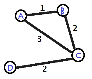
| Dijkstra | B – Path | COST | C – Path | COST | D – Path | COST |
| A | A-B | 1 | A-C | 3 | – | ∞ |
| A,B | A-B | 1 | A-C | 3 | – | ∞ |
| A,B,C | A-B | 1 | A-C | 3 | A-C-D | 5 |
| A,B,C,D | A-B | 1 | A-C | 3 | A-C-D | 5 |
| Bellman-Ford | B – Path | COST | C – Path | COST | D – Path | COST |
| 1 | A-B | 1 | A-C | 3 | – | ∞ |
| 2 | A-B | 1 | A-C | 3 | A-C-D | 5 |
| 3 | A-B | 1 | A-C | 3 | A-C-D | 5 |
Until Next Time,

Nitemice
Related articles
- Crammer’s Guide – Y01S01: Computer System Fundamentals (nitemice.com)
- Crammer’s Guide – Y01S01: Database Theory (nitemice.com)
- Crammer’s Edition – Maths for Computing (nitemice.com)
- Crammer’s Guide – Y01S01: Java Programming 1 (nitemice.com)
